Tuesday, 17 November 2026

Moving Megaliths With A Hurdle Trackway

Most reconstructions of how the Stonehenge sarsens were moved fall into two families: sledges on rollers, and sledges on a fixed timber track or greased rails. Both face the same problem on soft ground. A heavily loaded runner or roller presses on a narrow strip, and on wet clay-with-flints or waterlogged topsoil it sinks. This post proposes a third option, using a technology the Neolithic is known to have had: woven hazel hurdles, laid as portable ground-pressure mats, greased on the top face, and leapfrogged from the rear of the sledge to the front as it advances.

The aim here is not to show that it was done, but whether it could work: whether a hurdle that two people can carry survives a 25-tonne load, and whether the numbers for crew, pace and materials are realistic.

Neolithic hurdles

Woven panels of coppiced hazel are well attested in the Somerset Levels. The Neolithic hurdle trackway at Walton Heath was published by Coles and Orme (1977). Making them required skilled hurdle-making, managed coppice and a habit of laying hurdles as walkways over soft ground. Using them to carry a load is a small step from that: a short length of portable trackway, rather than a permanent one.

The method

A sarsen of about 25 t is lashed to an oak sledge with two runners, each 6 m × 0.3 m, set 1.4 m apart, with upturned noses. Hurdles of about 2.4 m × 1.2 m are laid across the line of travel, butted end to end, with tallow on the top face along the strips the runners will cross. Each 1.2 m the sledge advances, the rearmost hurdle is unloaded. A pair lifts it, carries it forward beside the track, lays it against the leading hurdle, and greases it again. Ten hurdles are in use at any one time: six under the runners, two laid ahead and two being carried.

Figure 1. Side elevation, schematic.

Figure 2. The relay cycle in plan.


Animation of the relay cycle, side and plan views.

The track moves with the stone. Nothing has to be laid along the whole route, and the heaviest item anyone lifts is a hurdle of about 40 kg.

Ground pressure

The total load, stone and sledge, is about 27.5 t (270 kN). On bare runners the contact area is 3.6 m², a mean pressure of about 75 kPa. On the hurdles the load spreads over the panels beneath the runners: about 19 kPa if the hurdles behaved as rigid mats, about 28 kPa allowing for the flexibility of the wattle. That is close to the pressure of a person standing (about 21 kPa).

The undrained bearing capacity of a surface strip footing is about 5.14 cu. For very soft, waterlogged ground (cu ≈ 12 kPa) that gives about 62 kPa, and for soft ground (cu ≈ 20 kPa) about 103 kPa. Bare runners exceed the first and would plough in. On hurdles the factor of safety is about 2–3 even on the weakest ground considered.

Figure 3. Contact pressure against ultimate bearing capacity.

Will the hurdles survive?

Crushing. With rods about 25 mm in diameter at about 30 mm spacing, the two runners cross about 400 rods, roughly 0.67 kN per crossing. If only one in four crossings bears its full share, because the weave makes the surface uneven, that rises to about 2.7 kN. Taking the compressive strength of hazel across the grain as about 7 MPa, the crushed contact band is about 1.3 mm wide. Crushing does not limit the method.

Bending. Bending does. A green hazel rod of 25 mm (modulus of rupture about 50 MPa) bridges a void under the runner of only about 0.1 m at the uneven-bearing load, and about 0.45 m at the mean load. Hollows along the line of travel are bridged by the stiff oak runner. Ruts running parallel to the track are not, and they would have to be filled with turf or brushwood before the hurdles were laid.

Staying in place. The method only works if the hurdle stays still while the runner slides over it. The runner drags the hurdle forward with a force of μtopN, and the ground resists with μground(N + w). With wattle bedded into turf (μground ≈ 0.55), ground grip exceeds the greased drag by about 4.2× at nominal friction (0.13), 3.1× with worn grease (0.18), and 1.6× even on dry wattle (0.35). This is why only the top face is greased. Tallow on the underside would undo the arrangement.

Figure 4. Rod loading and the force balance on a hurdle.

Crew and pace

The haul force is F = W(μ cos θ + sin θ). Taking a sustained rope pull of 0.3 kN per person, the crew for a 25 t sarsen on greased hurdles (μ ≈ 0.13, including resistance from the bumps of the weave) is about 120 on the level, about 160 on a 1 in 20 slope and about 210 at 1 in 10. On dry wattle the figures are about 315, 360 and 400.

For comparison, in the 2016 UCL trial ten people pulled a 1.1-ton stone on a sycamore sledge over a track of silver birch logs, at about ten feet every five seconds (Archaeology; see also the earlier sarsen.org note). At the same 0.3 kN per person, that implies an effective friction coefficient of about 0.25, between the greased and dry values used here. That is a cross-check of order of magnitude, not a calibration.

Pace is set by the relay, not by the hauling. One relay (walk about 10 m, lift, lay, butt, grease) takes about 35 s. With three relay pairs taking turns, a hurdle is laid every 12 s or so, which gives about 370 m an hour. At six hours a day, the 25 km from West Woods to Stonehenge takes about 11 working days per stone.

Figure 5. Haul crew needed, and relay logistics.

Weak points

  • Wear. Over 25 km each of the ten hurdles in use would be loaded about 2,100 times. Abrasion of the rod crowns, not their strength, will set hurdle life. A reserve of 30–50 hurdles, with a team making replacements, is the realistic requirement.
  • Lubricant. Assuming a 0.2 mm film on the runner strips, with 10–30 per cent lost on each pass, tallow consumption is about 16–49 kg/km, or 0.4–1.2 t per 25 km trip. This is the least certain number in the analysis. If the true loss rate sits at the top of the range, the supply of grease, rather than the supply of people, could limit how often stones were moved.
  • Ground preparation. Ruts and hollows across the line of the runners must be filled before laying.
  • Steering and slopes. A sledge on greased hurdles slides sideways as easily as forwards. On a cross-slope it will drift, so it needs guide ropes or levers. Downhill it needs a braking crew on rear ropes.

What an experiment should measure

Each of the uncertain numbers can be tested at modest scale: a single loaded runner of, say, 2–3 t on two or three hurdles. Four measurements would constrain the analysis:

  1. the haul force on greased and dry wattle, which gives μtop directly;
  2. whether, and at what force, a loaded hurdle creeps over turf, which gives μground;
  3. grease loss per pass, by weighing;
  4. wear on the rod crowns after a few hundred passes.

Assumptions

ParameterValue
Stone + sledge25 t + 2.5 t
Runners2 × 6.0 m × 0.30 m, gauge 1.4 m
Hurdle2.4 × 1.2 m, ~40 mm thick, ~25 mm rods; ~39 kg
Friction, greased top0.08 (fresh) – 0.13 (nominal) – 0.18 (worn)
Friction, dry wattle0.35
Friction, hurdle on turf0.55
Hazel, compression across grain / MOR (green)~7 MPa / ~50 MPa
Rope pull per hauler, sustained0.3 kN
Undrained shear strength, very soft / soft ground12 / 20 kPa
Relay cycle~35 s; three pairs

All values are assumptions for estimating orders of magnitude, not measurements.

References

Coles, J.M. and Orme, B.J. 1977. Neolithic hurdles from Walton Heath, Somerset. Somerset Levels Papers 3, 6–29.
People Could Have Pulled Bluestones to Stonehenge. Archaeology, 27 May 2016.

Sunday, 15 November 2026

Where the ice stopped: the Bristol Channel at the Last Glacial Maximum

This post is the companion to the short film Where the ice stopped, which animates the BRITICE-CHRONO model of the last ice sheet in the Celtic Sea and Bristol Channel from 31,000 to 15,000 years ago. The measurements behind it, with sources, follow.

Five published reconstructions of the last British–Irish Ice Sheet give the position of the ice margin in the Celtic Sea and Bristol Channel between 31,000 and 15,000 years ago. Their deposited GIS data are drawn together and measured in an interactive map: Bristol Channel LGM ice limits. No reconstruction carries Irish Sea ice across the north coast of Cornwall, Devon or Somerset. One margin is drawn along that coast. The others end between 4 and 24 km from it at their closest.

Open the interactive map: Bristol Channel LGM ice limits.


The reconstructions

  • BRITICE-CHRONO empirical reconstruction (Clark et al. 2022): minimum, optimum and maximum ice extents at thousand-year steps from 31 to 15 ka.
  • BRITICE-CHRONO model reconstruction (same paper): an ice-sheet model nudged towards the empirical limits, deposited as grids of about 2.5 km.
  • DATED-1 (Hughes et al. 2016): minimum, most-credible and maximum extents for the Eurasian ice sheets, with a census date of 1 January 2013.
  • Batchelor et al. 2019 (Nature Communications 10, 3713): a single best-estimate LGM outline within a Northern Hemisphere compilation.
  • PaleoMIST 1.0 (Gowan et al. 2021): global margins at 2,500-year steps.

These are three source families, not five independent tests. PaleoMIST takes its Eurasian margins from the DATED-1 most-credible lines, with intermediate slices interpolated. Batchelor et al. compile published outlines. BRITICE-CHRONO supplies both an empirical reconstruction and a model fitted to it. Reconstructions published only as figures, without deposited geometry, are not included.

Distance from the modern north coast

The coast was followed for 316 km from Land's End to Brean Down and sampled every 2 km. For each margin, the distance from each coastal point to the nearest ice was computed, using the union of all time-slices so that each margin is taken at its farthest reach.

Margin Closest approach Median distance offshore
BRITICE-CHRONO maximum boundat the coast1.6 km
BRITICE-CHRONO model, grounded ice3.7 km14.6 km
BRITICE-CHRONO optimum8.6 km21.7 km
Batchelor et al. 201914.8 km30.1 km
DATED-1 most credible18.5 km42.7 km
PaleoMIST 1.023.6 km75.3 km

The BRITICE-CHRONO maximum bound lies within 5 km of the shore along 89% of the coast measured. It overlaps 53 km² of land, 0.4% of the peninsula, as coastal slivers no more than 1.8 km deep at the sampled points. The optimum of the same reconstruction lies 8.6 to 41.5 km offshore.

The model grows ice on the South-West peninsula, 546 km² summed over all time-slices, but as separate upland ice on Dartmoor and Exmoor. It is not connected to the Irish Sea Ice Stream in any slice.

Lundy, Scilly and Fremington

Lundy separates the margins. The island lies inside the BRITICE-CHRONO maximum bound and inside the model's grounded ice, and 6.0 km outside the optimum. Rolfe et al. (2012) report 10Be exposure ages of 31.4–48.8 ka from the island and read them as glaciation before the LGM. Carr, Hiemstra and Owen (2017) argue that Lundy was not ice-covered in the Devensian.

The Isles of Scilly sit on the BRITICE-CHRONO empirical margin, within 0.1 km in all three versions. Smedley et al. (2017) date the ice limit on the northern islands to about 26 ka.

Fremington lies outside every margin in every time-slice. The nearest is the BRITICE-CHRONO maximum bound, 12.6 km away.

Sea level

Distances are measured to the modern coast because that is where the onshore evidence begins, and because it is the line the maximum bound follows. It was not the shoreline of the time. The shoreline of each date is taken from the glacio-isostatic palaeotopography published with the BRITICE-CHRONO reconstruction.

In that model the shoreline lies a median 47 km from the modern north coast at 31 ka. Crustal depression under the ice brings it to a median 19 km at 25 ka, and it withdraws to 52 km by 19 ka. At no date does it come within 5 km of the coast measured. A uniform lowering of sea level by 120 m would not reproduce this pattern.

A margin that follows the modern shoreline for most of 316 km therefore follows a line that was not the shoreline at any date in the reconstruction.

The same palaeotopography shows how much of each ice front that now lies under the sea stood on dry land. At 26 ka the figure is 37% for the BRITICE-CHRONO optimum, with the remainder in water of 48 m median depth, and 47% for the model. For the DATED-1 most-credible margin at 23 ka it is 5%.

Limits

  • Line-work in regional and hemispheric compilations is drawn at small scale. Differences of a few kilometres between margins, and between a margin and the coast, are within drafting precision.
  • The palaeo-shoreline is an output of a glacio-isostatic model tied to the BRITICE-CHRONO ice history. Beside the DATED-1, Batchelor and PaleoMIST margins it is indicative only.
  • The chronologies differ. DATED-1 places the Celtic Sea lobe in its 23 ka slice; BRITICE-CHRONO places the greatest extent in this area at 26 ka.
  • In the animation, flow direction is inferred from the modelled ice-surface slope. The deposited data give flow speed but not direction.

Notes on the film. The animation shows the BRITICE-CHRONO model reconstruction (Clark et al. 2022), deposited as thousand-year grids of ice thickness, surface elevation and surface speed at about 2.5 km; frames between slices are interpolated. Flow lines are particles moved down the slope of the smoothed modelled ice surface at a rate set by the modelled surface speed: the deposited data give speed, not direction. Land and sea at each date are from the same study's palaeotopography; the thin line is the modern coast. Relief: NOAA ETOPO 2022. Music: original.

Sources

  • Clark, C.D. et al. (2022). Growth and retreat of the last British–Irish Ice Sheet, 31 000 to 15 000 years ago: the BRITICE-CHRONO reconstruction. Boreas 51(4), 699–758. doi:10.1111/bor.12594. Data: doi:10.1594/PANGAEA.945729.
  • Hughes, A.L.C., Gyllencreutz, R., Lohne, Ø.S., Mangerud, J., Svendsen, J.I. (2016). The last Eurasian ice sheets – a chronological database and time-slice reconstruction, DATED-1. Boreas 45(1), 1–45. doi:10.1111/bor.12142. Data: doi:10.1594/PANGAEA.848117.
  • Batchelor, C.L. et al. (2019). The configuration of Northern Hemisphere ice sheets through the Quaternary. Nature Communications 10, 3713. doi:10.1038/s41467-019-11601-2. Data: osf.io/7jen3.
  • Gowan, E.J. et al. (2021). A new global ice sheet reconstruction for the past 80 000 years. Nature Communications 12, 1199. doi:10.1038/s41467-021-21469-w. Data: doi:10.1594/PANGAEA.905800.
  • Smedley, R.K. et al. (2017). New age constraints for the limit of the British–Irish Ice Sheet on the Isles of Scilly. Journal of Quaternary Science 32(1), 48–62. doi:10.1002/jqs.2922.
  • Rolfe, C.J., Hughes, P.D., Fenton, C.R., Schnabel, C., Xu, S., Brown, A.G. (2012). Paired 26Al and 10Be exposure ages from Lundy. Quaternary Science Reviews 43, 61–73. doi:10.1016/j.quascirev.2012.04.003.
  • Carr, S.J., Hiemstra, J.F., Owen, G. (2017). Landscape evolution of Lundy Island: challenging the proposed MIS 3 glaciation of SW Britain. Proceedings of the Geologists' Association 128(5–6), 722–741. doi:10.1016/j.pgeola.2017.06.005.
  • Base map: NOAA ETOPO 2022 relief; GSHHG 2.3.7 shoreline (Wessel and Smith 1996).

Map, measurements and code outputs: github.com/TimDaw37/bristol-channel-lgm-ice. Measurements made on 15 November 2026 from the data as deposited.

Saturday, 14 November 2026

The British Isles in relief: open LiDAR maps to download

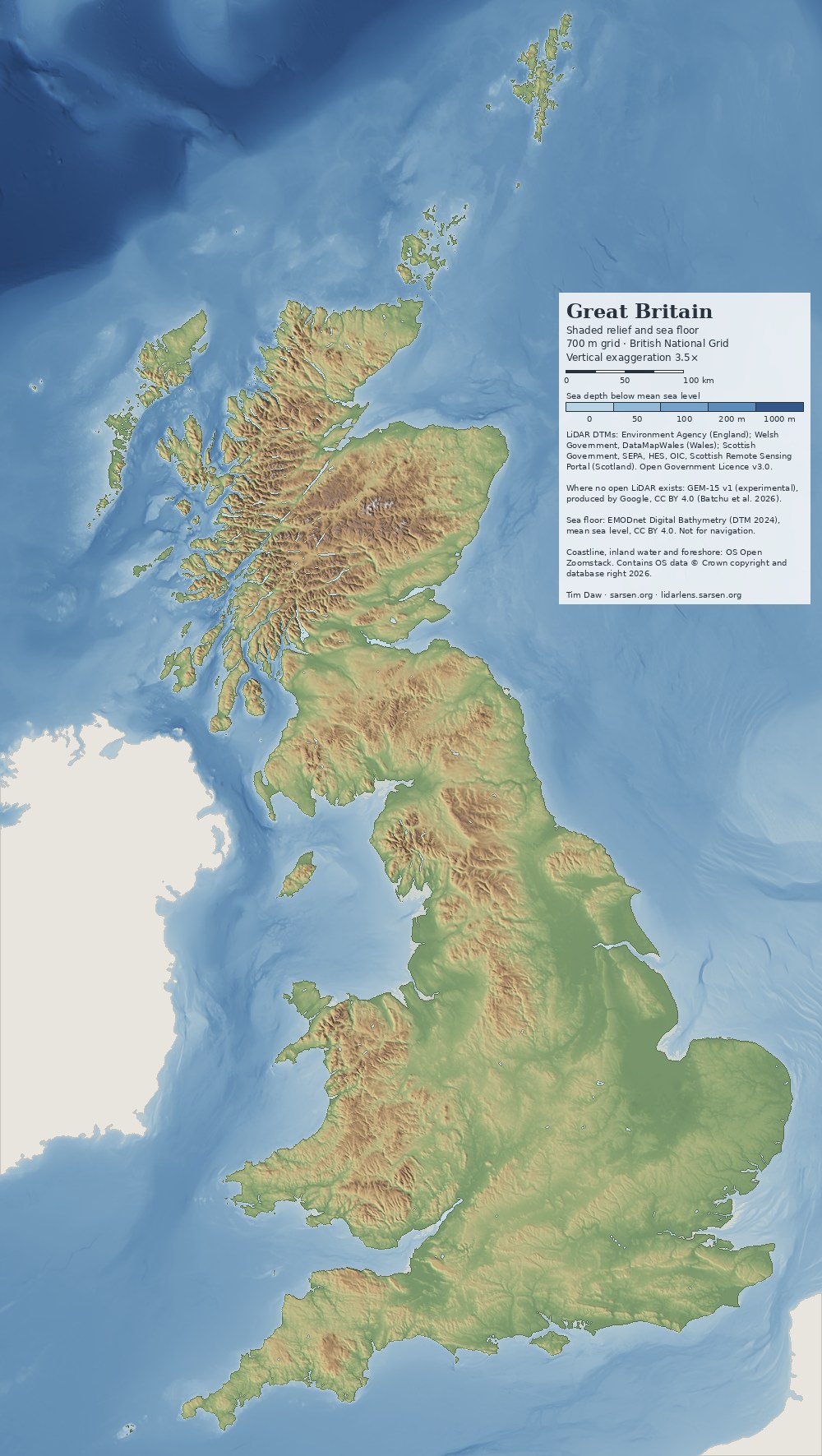
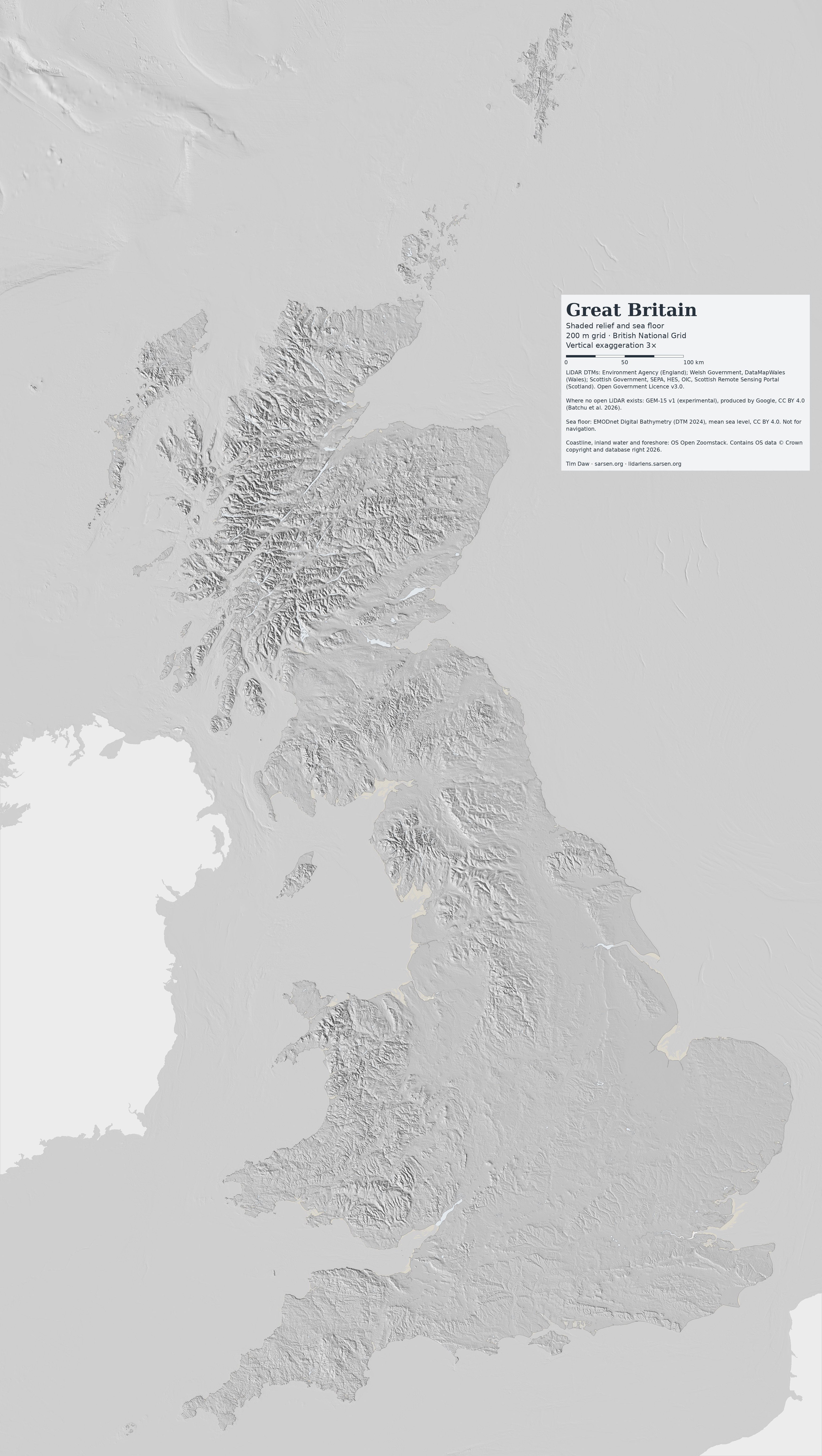
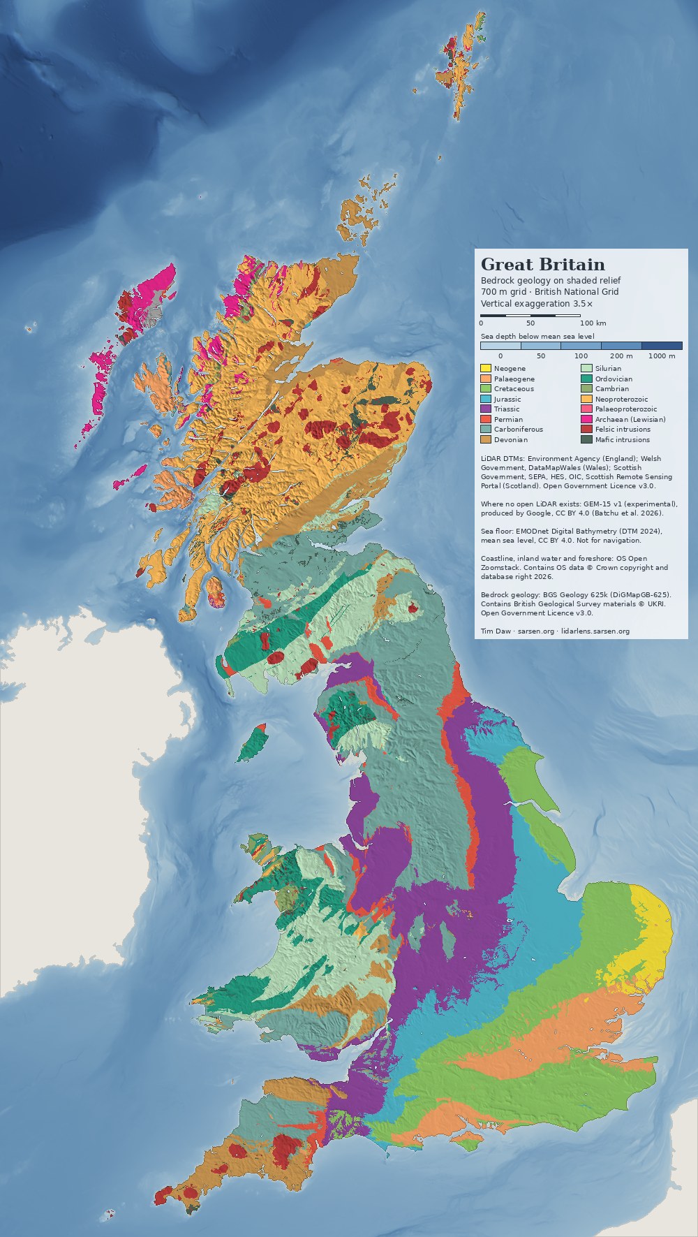
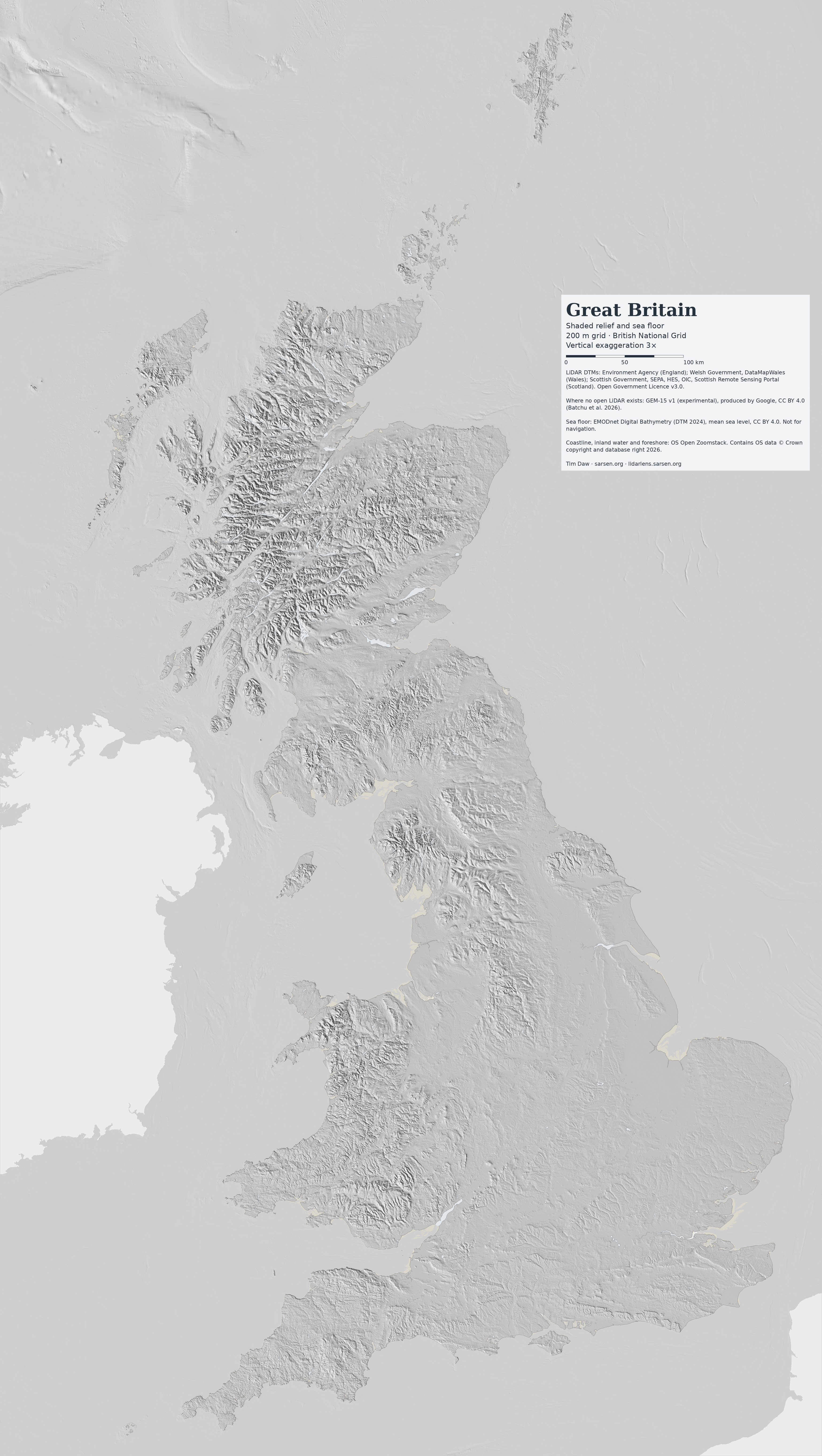
A shaded relief map of the whole of Great Britain and the surrounding sea floor, built from the same open LiDAR terrain models and EMODnet bathymetry that drive LiDAR Lens. It comes as ready-made images, as an interactive map that exports framed and credited images, and as base-map tiles for web maps. A second version lays BGS bedrock geology over the relief. Everything is free to reuse under CC BY 4.0.

Shaded relief map of Great Britain with a green-to-brown elevation tint, showing the Scottish Highlands, the Lake District, the Pennines, Snowdonia and the chalk and limestone scarps of southern England, with the sea floor shaded in blue by depth
Great Britain, shaded relief and sea floor, 700 m grid, British National Grid. Click for the 3500 px version.

Downloads

Version1000 px
700 m grid
3500 px
200 m grid
7000 px
100 m grid
ReliefJPGJPG · PNGJPG · PNG
Grey hillshadeJPGJPG · PNGJPG · PNG
Elevation tintJPGJPG · PNGJPG · PNG
Bedrock geologyJPGJPG · PNGJPG · PNG

The 7000 px versions print at about A1 (200 dpi) or A2 (300 dpi). Vertical exaggeration is 3.5×, 3× and 2.5× from the smallest size to the largest, enough to keep lowland scarps visible at each scale. Title, scale bar and data credits are printed on every image.

Map of Great Britain showing bedrock geology by period, coloured to the international chronostratigraphic chart and draped over shaded relief
Bedrock geology (BGS Geology 625k) by period, on shaded relief. Igneous intrusions are coloured by composition.

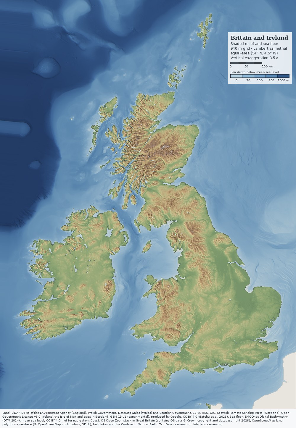
Britain and Ireland

Shaded relief map of Britain and Ireland with the surrounding sea floor shaded in blue by depth, from the Rockall Trough to the southern North Sea
Britain and Ireland, shaded relief and sea floor, Lambert azimuthal equal-area projection. Click for the 3500 px version.

Both islands are also mapped together on a Lambert azimuthal equal-area projection centred at 54° N, 4.5° W, which keeps areas true and distortion small across the two. Ireland and the Isle of Man are GEM-15. The open Irish LiDAR now in LiDAR Lens covers only a few per cent of the island and adds nothing visible at these scales. Outside Great Britain the coastline is the OpenStreetMap land-polygon line (mean high water), and the larger Irish loughs are from Natural Earth.

Version1000 px3500 px7000 px
Relief and sea floorJPGJPG · PNGJPG · PNG
Grey hillshadeJPGJPG · PNGJPG · PNG
Elevation and depth tintJPGJPG · PNGJPG · PNG

There is no combined geology version yet: BGS Geology 625k stops at the coast of Great Britain.

Make your own map

The interactive map uses the same data and rendering. It offers four styles (relief, grey hillshade, elevation tint, geology) and four colour schemes, with a multi-directional or single sun, adjustable sun direction and height, and adjustable vertical exaggeration. Inland water can be switched on or off. Any frame can be exported, as on screen or in A-series, square or 16:9, at up to 7200 px, with an editable title and the required credits. Tapping the map gives the grid reference, height and, in geology mode, the bedrock period. A link opens the same spot in LiDAR Lens at full 1 m resolution.

For web maps

Web Mercator tiles (zoom 5 to 11, sea floor included, Ireland and France transparent) are available in relief, grey and geology versions for Leaflet, MapLibre or OpenLayers:

<script src="https://timdaw37.github.io/gb-relief/gbrelief.js"></script>
GBRelief.layer('relief').addTo(map);   // or 'grey', 'geology'

For both islands, use 'relief-bi' or 'grey-bi'. Template: https://timdaw37.github.io/gb-relief/tiles/{style}/{z}/{x}/{y}.webp. Full details are in the repository.

Data and method

Terrain. The terrain comes from 1 m open LiDAR digital terrain models. England is covered by the Environment Agency LiDAR Composite DTM. Wales is covered by the Welsh Government LiDAR DTM, via DataMapWales. Scotland is covered by Scottish Government, SEPA, HES and OIC LiDAR, via the Scottish Remote Sensing Portal. The data were resampled to about 90 m and reprojected to the British National Grid at 100 m. Parts of the Highlands and Islands and the Isle of Man have no open LiDAR. There the terrain is GEM-15 v1, Google's experimental 15 m bare-earth model (Batchu et al. 2026). Against the Scottish LiDAR its median per-tile offset is −0.09 m, so the two join without a visible step at this scale.

Sea floor. Offshore, the surface is the EMODnet Digital Bathymetry DTM 2024 (mean-sea-level version, about 115 m cells, CC BY 4.0), as prepared for LiDAR Lens, and is shaded in the same way as the land under a blue depth tint. The overdeepened glacial basins of the Inner Hebrides and the Firth of Lorn, the linear tidal sandbanks off East Anglia, and the continental slope into the Rockall Trough (deeper than 1300 m at the north-west corner of the frame) all show. EMODnet compiles surveys of different ages and quality and fills the gaps between them, so straight lines and steps can be survey artefacts rather than landforms. Depths are relative to mean sea level, not Ordnance Datum, and are not for navigation.

Coast and water. The Environment Agency composite includes LiDAR returns over the sea and in estuaries, at about −4 to +2 m. Left in, they produce false land, such as a strip joining Lundy to the Devon coast. Land is therefore clipped to mean high water using OS Open Zoomstack, which also supplies inland water bodies and foreshore.

Shading. Slopes are taken from central differences. The light is a weighted four-direction sun: 315° at weight 0.5, 270° and 0° at 0.2 each, and 225° at 0.1, all at 40° elevation. This brings out ridges and scarps that run north-west to south-east, parallel to the main light, which a single north-west light leaves flat. The elevation tint runs from green lowland to brown upland, with pale summits above 1100 m.

Geology. The bedrock is BGS Geology 625k (DiGMapGB-625), coloured by period with the International Commission on Stratigraphy chart colours. Felsic and mafic intrusions are shown separately. At 1:625,000 the geological boundaries are generalised and coarser than the relief beneath them.

Resolution. At these scales the 1 m LiDAR adds little beyond consistency and the absence of interpolation artefacts. A national relief map at 100 m built from OS Terrain 50 would differ little. The LiDAR matters at field scale, which is what LiDAR Lens shows.

Licence and credit

The maps and tiles are free to use under CC BY 4.0. Credit "GB Relief, Tim Daw (sarsen.org)" and keep the data credits:

LiDAR DTMs: Environment Agency (England); Welsh Government, DataMapWales (Wales); Scottish Government, SEPA, HES, OIC, Scottish Remote Sensing Portal (Scotland). Open Government Licence v3.0. GEM-15 v1 (experimental), produced by Google, CC BY 4.0. Sea floor: EMODnet Digital Bathymetry (DTM 2024), CC BY 4.0, not for navigation. Contains OS data © Crown copyright and database right 2026. Britain-and-Ireland versions: coastline outside Great Britain © OpenStreetMap contributors (ODbL); Irish lakes and the Continent from Natural Earth. Geology versions: contains British Geological Survey materials © UKRI, Open Government Licence v3.0.

EMODnet Bathymetry Consortium 2024. EMODnet Digital Bathymetry (DTM 2024). doi:10.12770/cf51df64-56f9-4a99-b1aa-36b8d7b743a1.

Batchu, V.V., Neumann, M., Li, T., Allen, B., Zhang, J. and Van Arsdale, C. 2026. GEM-15: Global surface and terrain elevation models (15 meters) from sub-meter optical stereo imagery. EarthArXiv preprint, not peer reviewed. doi:10.31223/X55N75.

Thursday, 12 November 2026

LiDAR Lens goes outdoors: field mode for walkers


LiDAR Lens now has a second face. Alongside the full research view (now called Lab) there is a stripped-down Field mode built for a phone held in one hand on a footpath: where am I, where is the earthwork, which way do I walk, and what is it when I get there.

Open it at lidarlens.sarsen.org/?ui=field, or switch between Field and Lab with the toggle at the top of the screen in either view.

What Field mode shows

The screen carries a search box (place, postcode or grid reference), zoom buttons and a single control panel at the bottom. Everything else in Lab — the fifteen visualisations, sliders, data layers and analytical tools — is hidden. The LiDAR fills the whole screen rather than sitting inside the lens circle.

Four view buttons cover what matters outdoors:

  • Hillshade — single low sun from the north-west, the conventional reading of earthworks.
  • VAT — the Combined VAT visualisation (Kokalj & Somrak 2019), blending hillshade, slope, openness and sky-view; better for low banks and ditches that a single sun misses.
  • Old map — the Ordnance Survey six-inch map (1888–1913) over the aerial photograph, useful for field boundaries, lost tracks and antiquarian annotations.
  • Aerial — the aerial photograph alone, for orientation against hedges, gates and buildings.

Coverage is the whole of Great Britain where 1 m LiDAR exists: the Environment Agency composite DTM for England, the Welsh Government DTM for Wales and the Scottish Remote Sensing Portal data for Scotland, all Open Government Licence and fetched live.

Finding a monument

  1. Set a target. Tap ◎ Target, then tap the feature on the map — or search for a place or grid reference. The target's grid reference appears in the panel.
  2. Allow location. The phone's GPS position is shown on the map and updated continuously. With a fix, the panel gives the distance and compass bearing from you to the target.
  3. Use the arrow. By default the arrow is drawn on a north-up map. Tap Use compass and the arrow turns with the phone, so it points the way to walk. On an iPhone this needs permission for motion and orientation, asked for the first time the button is pressed.
  4. Recentre. Panning the map stops it following you. Recentre returns to your position (framing the target too when it is close) and resumes following.
  5. Arrival. Within about 25 m of the target the panel reports that you are there; the threshold widens to as much as 50 m when the GPS fix is poor.
  6. What is it? Lists the heritage records within 30 m of the target, or of your position if no target is set: Historic England (National Heritage List and Aerial Investigation and Mapping) in England, Cadw and Coflein in Wales, and Historic Environment Scotland and Canmore in Scotland, with links to each record and Creative Commons photographs from Geograph where they exist. Measure this feature from the DTM gives its dimensions from the LiDAR.
  7. Done. Clears the target and leaves the map where it is, for looking at the LiDAR around you.

The target is stored in the page address, so a link copied from the browser opens with the same target set — a simple way to send someone a barrow to find.

Putting it on your phone's home screen

Field mode is set up as an installable web app. Added to the home screen it gets its own icon, is named LiDAR Field, opens straight into Field mode and runs full screen without the browser's address bar.

iPhone and iPad (Safari)

  1. Open lidarlens.sarsen.org/?ui=field in Safari.
  2. Tap the Share button (the square with an upward arrow).
  3. Scroll down and tap Add to Home Screen.
  4. Keep the name LiDAR Field or change it, and tap Add.

Recent versions of iOS also offer Add to Home Screen from the share menu in Chrome and Edge.

Android (Chrome)

  1. Open lidarlens.sarsen.org/?ui=field in Chrome.
  2. Tap the ⋮ menu at the top right.
  3. Tap Add to home screen (shown as Install app on some phones) and confirm.

Location permission. If the panel reads Location blocked, the browser has refused GPS access to the site. On iPhone: Settings → Privacy & Security → Location Services → Safari Websites, set to While Using the App with Precise Location on. On Android: in Chrome, tap the icon to the left of the address, then Permissions → Location → Allow. Tap Retry in the panel afterwards. The map and target work without location; only your position and the distance and bearing are lost.

Before you go

  • Signal. LiDAR tiles and records are fetched as you look and kept in the browser's cache, so ground already viewed reloads instantly. Browsing the walk at home on the phone over Wi-Fi is the best preparation for a valley with no signal. This is a cache, not a guaranteed offline map: an area not viewed beforehand will not load without a connection.
  • Access. Field mode does not show rights of way. Check the route in Lab beforehand, where the public footpaths, bridleways and byways layer and CRoW access land can be switched on. Many features on the LiDAR lie on private land.
  • Bare earth. The model is a terrain model with trees, hedges and buildings removed. A bank clear on screen may be under scrub on the ground.
  • Scheduled monuments. Looking is fine; metal detecting, digging or driving on them is not.
  • GPS accuracy. A phone in open country is typically good to a few metres, worse under trees or beside steep slopes. Use the target to get close, then the ground itself.

The code is open source on GitHub. Faults can be reported from the Report a fault link in Lab, which fills in the browser details automatically.


Saturday, 7 November 2026

Alfred and the Danes: an animated campaign map, 865–899

The Danish wars of 865–899 are documented almost entirely by one source tradition: the Anglo-Saxon Chronicle, Asser's Life of King Alfred (which follows the Chronicle closely for these years) and Æthelweard's Latin chronicle. Together they give a year-by-year itinerary of winter camps, sieges, named battles and treaties. They do not give routes, force sizes or, apart from Asser's account of Ashdown, tactical detail. Several of the named places cannot be located with confidence.

A new interactive map, Alfred and the Danes, 865–899, sets that itinerary out in 34 steps on a terrain base, from the arrival of the Great Army in East Anglia to Alfred's death in October 899. Each step is keyed to its annal and, where relevant, to Asser's chapter.

What the map shows

Danish movements are drawn in red and West Saxon movements in blue. Movements by sea, or where the starting point is not recorded, are dashed. Markers distinguish camps, battles, sieges, fortifications and treaties, and are coloured by which side held the field. The sources give places, not routes, so each line simply joins the recorded places in order and is schematic.

The background is built from:

  • OS Terrain 50 relief, with a tint deepening from 40 m to 260 m OD;
  • a mask of land below 6 m OD, as a rough indication of former wetland in the Somerset Levels and the Fens;
  • named main rivers from OS Open Rivers;
  • Roman roads from the Itiner-e dataset (static version 2024), drawn solid where the course is conjectured and dashed where it is hypothetical.

The Burghal Hidage burhs and the boundary in the Treaty of Alfred and Guthrum can be switched on. The coastline is modern. It does indicate though the 9th-century Wantsum Channel, the Limen estuary at Appledore and the earlier Fen edge.

Uncertain sites

Six of the named places are disputed: Ashdown, Meretun, Cynuit, Egbert's Stone, Iley and Ethandun. For each, the map draws the routes to a working identification, rings it, and shows the other candidates as open dots. Selecting another candidate redraws the routes. The candidates and their main proponents are:

  • Ashdown (871). Æscesdun was a name for the Berkshire Downs as a whole. Candidates are Kingstanding Hill near Moulsford, Lowbury Hill, Thorn Hill near Compton and, on antiquarian grounds, White Horse Hill. Asser's single stunted thorn tree does not narrow the choice.
  • Meretun (871). Candidates are Martin (Hampshire), Marten (Wiltshire), Marden (Wiltshire), Merdon near Hursley, and Merton in Oxfordshire or Surrey. None is preferred in the literature, and the working point is for display only.
  • Cynuit (878). Asser names the fort; the Chronicle says only "in Devon". Candidates are Countisbury, Cannington Camp, Kenwith near Bideford and Castle Hill near Beaford. Historic England treats Cannington as the accepted site, although it lies in Somerset.
  • Egbert's Stone and Iley (878). The Chronicle places Egbert's Stone east of Selwood. Proposed sites include Kingston Deverill, Kingsettle Hill, Penselwood and Willoughby Hedge. Iley follows the English Place-Name Society's identification with Iley Oak, the lost meeting-place of Warminster and Heytesbury hundreds.
  • Ethandun (878). Edington, Wiltshire is the consensus identification, with the fighting placed on or below the escarpment near Bratton Camp. The Somerset Edington on the Poldens remains a minority alternative.

The Edington march

The 878 campaign gets its own day-by-day sequence at larger scale, because the Chronicle gives an unusually tight itinerary. Alfred leaves Athelney in the seventh week after Easter and rides to Egbert's Stone, where the men of Somerset, Wiltshire and part of Hampshire meet him. After one night he moves to Iley, and after a second he moves at dawn to Ethandun and fights. Asser adds the pursuit to the Danish fortification and the fourteen-day siege, which ends with hostages, oaths and Guthrum's baptism at Aller.

The panel computes straight-line distances for each leg from whichever candidates are selected. With Kingston Deverill and Eastleigh Wood as working sites, the legs are:

  • Athelney to Egbert's Stone: 50 km
  • Egbert's Stone to Iley: 8 km
  • Iley to Ethandun: 10 km
  • Ethandun to Chippenham: 21 km

The first leg ranges from about 40 km (Kingsettle Hill) to 55 km (Willoughby Hedge), depending on the candidate. These are minima, not road distances. On any of the eastern candidates, the march runs off the Levels, over the Selwood ridge and up onto the chalk, so the final approach to the Edington escarpment comes from the south-west across the Plain.


Chronology

The Chronicle's year in this period began in autumn or at Christmas, so modern dates for the early annals can fall up to a year before the annal number. The battle of Reading, for example, belongs to the turn of 870–871 under annal 871. For the 890s the map follows the corrected chronology; manuscript A numbers several of those annals a year later.

Use

The map steps or plays through the campaigns, and can be panned and zoomed. Each step has its own link, for example #step-878f for Ethandun. Layers for rivers, low ground, Roman roads, the schematic Ridgeway and Harrow Way, burhs and alternative sites are under Layers.

The code and data are on GitHub. Corrections to site identifications, and further candidates with references, are welcome.

Sources

Friday, 6 November 2026

Heritage at Risk 2026: still at risk, on the nation's own land


Historic England has just published its 2026 Heritage at Risk Register. It lists 4,991 entries: 197 were added this year and 85 came off for positive reasons. Those headline totals look like steady progress. The picture is very different when you look at land owned by the Crown, meaning the Crown Estate, the Duchy of Cornwall and other Crown bodies.

The Crown's list is getting longer

In 2025, 97 Crown-owned entries were on the register. In 2026, all 97 are still there, and none has been rescued. Ten more have been added, bringing the total to 107. Nine of the new ones are on the Isles of Scilly, where 46 of the islands' 50 at-risk entries are Crown land, and the tenth is Warren Farm Barn at Chadwell Heath.

These are not recent problems. Sixty-eight of the Crown's entries have been at risk since at least 2013. Historic England records 79 of the 107 as declining, 20 as stable and only 8 as improving.

On our doorstep: the Marlborough Downs

Six Crown-owned monuments on the Marlborough Downs, near us and near Avebury, are still on the list. They are barrows and a farmstead on Bishops Cannings Down, Horton Down and Beckhampton, and they range from Kitchen Barrow to the Horton Down barrow cemetery. All six have been at risk since at least 2013, and all six are declining. Across the wider Marlborough Downs, 36 sites are at risk, down from 38 last year.

The National Trust and Wiltshire

For comparison, 64 entries are on National Trust land, up from 61. All four new ones are on Lundy, and one, the Quarterwall cottages on Lundy, came off. Forty-two of the Trust's entries have been at risk since at least 2013.

Wiltshire and Swindon together have 144 entries at risk, down from 150. Eight came off, including the henge and barrows southwest of Fox Covert on the boundary of Bishops Cannings and Avebury, and the Liddington Warren long barrow. That is welcome news. One genuinely new entry was added, the medieval cross in St Mary's churchyard, Purton.

What should happen

The Crown is not a struggling private owner. It is the nation's own landholder, with professional land agents and considerable income. Yet it has not removed a single monument from the at-risk register this year, its list has grown by ten, and most of its entries are getting worse.

I would like to see a simple step taken: for every Crown and Duchy entry on the register, a published plan and a target date for getting it off.

You can explore the sites yourself on my Heritage at Risk map, which has a slider covering 2013 to 2026.

Figures come from Historic England's 2026 Heritage at Risk spreadsheet and map data. National Trust figures count register sites that overlap Trust land by at least 10%.

Thursday, 5 November 2026

The Hunt for the Altar Stone Source - the video

The Youtube video

Altar Stone diagnostic toggle map


The Altar Stone diagnostic toggle map is an interactive screen of candidate source areas for the Stonehenge Altar Stone. Each published diagnostic is a layer that can be switched on or off, so the effect of any one test on the list of surviving candidates can be seen directly. The code and data are in the GitHub repository.

What it plots

The map covers 85 candidate places: Ba/Rb geochemical clusters across Britain and Ireland, plus named sites with published measurements. An Old Red Sandstone underlay from the BGS Geology 625k dataset shows where the outcrop lies. Fourteen layers score each place:

  • L0–L9: the baseline screen, covering barium and Ba/Rb geochemistry, mineralogy, zircon ages, thermal maturity and related published criteria.
  • L10 and L11: a strontium ceiling and the Sr/Ca ratio, applied only where rock Sr has been measured.
  • U1 and U2: chrome spinel (CZi) and illite/smectite expandability, from Pirrie et al. (2026). Both start off.

How to read it

A place is a match only if it fails none of the layers switched on. Each layer has strict and relaxed settings where the evidence allows. Untested is not failed: a place with no data for a layer stays open on that layer. Presets switch one test or group off at a time (leave-one-out), which shows how much each test contributes, and the preset "CZi + I/S ON (Pirrie et al. 2026)" applies the new chrome spinel and clay results.

Several things are deliberately not scored: the ORS between the Midland Valley and the Welsh Borders, the Lanark Basin, Carboniferous sandstones such as the Clifton Rock, and the Sr–Nd isotope result, because the evidence is missing or has no comparison data. The Latheron–Niandt cool sliver is drawn as schematic only.

Limits

The map is a screening tool. A place that survives is untested or consistent with the evidence so far, not identified as the source, and exclusion by elimination covers only the ground that has been sampled. Corrections and additional data are welcome.

The Pirrie, Bevins, Ixer et al paper that prompted the latest update is discussed in a separate post.

Paper: Pirrie, D., Bevins, R.E., Ixer, R.A., Pearce, N.J.G., Turner, P., Power, M.R. et al. 2026. Searching for the origin of the Stonehenge Altar Stone: new sedimentological, petrographical, mineralogical, geochemical and isotopic constraints. Journal of the Geological Society 183, jgs2026-090. doi:10.1144/jgs2026-090

Searching for the origin of the Stonehenge Altar Stone

A paper now published in the Journal of the Geological Society reopens the question of where the Stonehenge Altar Stone came from. Pirrie, Bevins, Ixer and ten further co-authors give the most detailed description of the stone to date: sedimentology, petrography, heavy minerals, clays, geochemistry and isotopes. Their conclusion is that no outcrop of Old Red Sandstone (ORS) examined so far matches it on every count, and that its provenance "has yet to be determined with confidence".

Paper: Pirrie, D., Bevins, R.E., Ixer, R.A., Pearce, N.J.G., Turner, P., Power, M.R. et al. 2026. Searching for the origin of the Stonehenge Altar Stone: new sedimentological, petrographical, mineralogical, geochemical and isotopic constraints. Journal of the Geological Society 183, jgs2026-090. doi:10.1144/jgs2026-090
Data: figshare doi:10.6084/m9.figshare.33993488.v1

Fig. 1. (a) Map of the UK showing the location of Stonehenge and the distribution of non- marine sediments of the Old Red Sandstone. (b) Plan showing the position of the Altar Stone within the Stonehenge monument (c) Photograph looking towards the SW; the Altar Stone (arrowed AS) is lying mostly underneath the two large sarsen stones. (c)
Source: photograph by Adam Stanford.

Where the question stood

The Altar Stone is a block of about six tonnes (4.9 × 1 × 0.5 m) lying flat beneath fallen sarsens 55b and 156. For a century it was assigned to the Cosheston beds of West Wales, following H.H. Thomas in 1923. Bevins and colleagues refuted that in 2020, and in 2023 they excluded the Anglo-Welsh Basin as a whole: of 58 samples, all but four failed on geochemistry and the remaining four on mineralogy. In 2024 Clarke et al. (Nature) dated zircon, apatite and rutile grains from Altar Stone debitage and proposed the Orcadian Basin of NE Scotland. Clarke et al. (2026) later suggested Caithness or the Inverness–Black Isle area as the most likely sources.

What the new paper adds

The study combines previously published in-situ pXRF on the three exposed areas of the stone with new laboratory work on three museum fragments (MS1–MS3): automated SEM-EDS mineralogy, X-ray powder diffraction of bulk rock and clay fractions, cathodoluminescence, C–O isotopes and colour. Sr–Nd isotopes were measured on MS1 and MS2. The characteristics that emerge are:

  • A bedding plane. Low-angle illumination in 2024 showed climbing ripples and slumped foresets on the exposed surface. If it is a bedding plane, the bed was at least 0.5 m thick and extended at least 4.9 m. There is no cleavage, and no petrographic sign of palaeosols or near-surface soil formation.
  • Chrome spinel. The chrome spinel:zircon index (CZi) is 35.9–38.6 in the three fragments. In ORS comparison data it averages 1.3 on Orkney (n = 35), 1.4 on the Tarbat peninsula, Inner Moray Firth (n = 42), 0.4 on Foula and Shetland (n = 13) and 0.2 in the Lower ORS of Pembrokeshire (n = 32).
  • Clay minerals. The clay fraction contains illite, mixed-layer illite/smectite, kaolinite, chlorite and tosudite. The illite/smectite is about 20% expandable in all three fragments. Expandability falls with burial and heating, and the ORS of Caithness and Orkney is below 10%, which excludes them. The clays alone would not exclude parts of the Moray Firth.
  • Barium. Dispersed baryte cement gives pXRF Ba of about 1000–5500 ppm (mean 2758 ppm), linearly related to Sr. This separates the stone from ORS analyses in Wales and Orkney.
  • Sr–Nd isotopes. 87Sr/86Sr is 0.7163–0.7169 and 143Nd/144Nd 0.5119–0.5121. Published Carboniferous sandstones (Leng et al. 1999) have either higher Nd or higher Sr isotope ratios, so there is little overlap. The Nd range of the ORS overlaps closely, but no ORS Sr isotope data exist, so the comparison cannot be taken further. The authors conclude that an ORS source is more likely than a Carboniferous one.
  • Diagenesis. Pore-filling kaolinite pre-dates significant compaction; baryte post-dates compaction; both pre-date the dominant poikilotopic burial calcite cement.

What is excluded

  • West Wales and the Anglo-Welsh Basin: excluded on earlier geochemistry and mineralogy, and in this paper by the absence of chrome spinel in West and South Wales and Somerset. Welsh Borderland tosudite occurrences are excluded on Ba.
  • Orkney and Caithness: excluded on clay expandability. Chrome spinel is also scarce in the Orkney, Tarbat and Shetland samples; Caithness itself was not sampled for it.
  • Moray Firth / Tarbat: compatible on clay, excluded on chrome spinel.
  • Midland Valley ORS: excluded on abundant lithic grains (Phillips 2007). In the NE Midland Valley, the Stonehaven and Arbuthnott groups have too little I/S expandability, and the zircon populations of the Dunnottar–Crawton to Strathmore groups differ. The Strathmore Group clays are comparable, but its zircons and the texture of its tosudite are not.
  • Southern Uplands: chrome spinel is common in the Lower Palaeozoic sandstones, but the Altar Stone contains kaolinite, which indicates it has not undergone low-grade metamorphism.
  • Late Carboniferous–Triassic of south-central Britain: no Variscan-age zircons in the Altar Stone.

What remains open

  • The ORS between the Midland Valley and the Welsh Borders, where modern heavy-mineral and zircon data are virtually absent.
  • Areas with Ba anomalies in stream-sediment geochemistry, including the Lanark Basin and the Fintona Basin of Northern Ireland. The paper reports no chrome spinel, zircon or clay data for the Lanark Basin.
  • Carboniferous sandstones recycled from Caledonide sources, such as the chrome-spinel-rich Clifton Rock of the Pennine Basin. Its zircon pattern differs (a large Early Palaeozoic peak, no Neoproterozoic group) and the Sr–Nd data favour the ORS, but the authors do not exclude it.

The diagnostic toggle map


These tests can be switched on and off in my Altar Stone diagnostic toggle map. Nothing to do with the paper or authors, I have just updated it with their data.  Each test is a layer: Ba/Rb screening, K-feldspar, zircon, clay and thermal maturity, strontium (L10, L11), and the chrome spinel (U1) and clay expandability (U2) results of Pirrie et al. The Pirrie layers start off; the preset "CZi + I/S ON (Pirrie et al. 2026)" switches both on. A place survives only if it fails none of the layers switched on, and untested is not the same as failed. Leave-one-out presets show how much each test contributes. The areas listed above as open, and the Sr–Nd result, are not scored on the map.

Relation to the NE Scotland proposal

The paper accepts the zircon, rutile and apatite ages of Clarke et al. and a Laurentian source for the heavy minerals. The argument is that the same age pattern can be shared by several basins, so ages alone cannot identify an outcrop, and that once chrome spinel, clays and barium are added the Orcadian candidates fail. Bevins and Ixer co-authored the 2024 Nature paper, so this is in part a team revising its earlier interpretation. The authors also regard the glauconite reported in one fragment by Clarke et al. (2026) as probably a misinterpretation of SEM-EDS spectra, and caution against relying on a single youngest zircon age.

Caveats

  • Three fragments. The new analyses are on three small museum fragments, and the Sr–Nd data on two. Their attribution to the Altar Stone rests on earlier pXRF and petrographic comparison, because the stone itself cannot be sampled.
  • Comparison data. The Pembrokeshire CZi value is from unpublished data, and the Orkney, Tarbat and Shetland values come from earlier compilations.
  • Elimination, not identification. "No match found" covers only the ground that has been sampled. Large areas of ORS have no modern heavy-mineral or zircon data.
  • Coarse Ba screening. National stream-sediment Ba maps are low resolution and can be distorted by historic mining.
  • Sr/Ca. Surface pXRF Ca on the in-situ stone is lower than on debitage, which the authors attribute to weathering of the calcite cement. Sr/Ca from the surface pXRF data is therefore biased upward and should be treated with caution.

Why it matters

The origin of the Altar Stone determines the journey and the contacts it implies. A Moray Firth or Caithness source suggests a long coastal voyage; a Lanark Basin source, routes via the Clyde and the Irish Sea; Fintona, a crossing from Ulster. Until a source is identified, the origin is a variable in route modelling, not a fixed point.

The characteristics reported in the paper define the tests a candidate source must pass: high Ba with baryte cement, CZi of about 36–39, illite/smectite about 20% expandable with tosudite, plagioclase far exceeding K-feldspar, and an ORS-type Nd isotope signature. Those are the tests for the next field campaign.

Figures and short quotations are from Pirrie et al. (2026); see the paper and its supplementary tables for the data.

Tuesday, 3 November 2026

Four Young Officers, Stonehenge 1938

This post is the companion to the short film Four Young Officers, made for Remembrance Sunday 2026: the four Royal Artillery subalterns who painted Stonehenge green in June 1938, and what became of them.

The night of 16 June 1938

By the summer of 1938 the four were serving with anti-aircraft and coast-defence units — Sherrard and Skinner at the School of Anti-Aircraft Defence, Biggin Hill; Peirce with the 22nd Anti-Aircraft Battery at the Royal Artillery experimental camp at Watchet; and Shearme at the Coast Artillery School, Shoeburyness — and had gathered at the School of Artillery, Larkhill, three miles north of Stonehenge, for a gunnery course. On the night of Thursday 16 June, after a mess guest night, they took green line-marking paint from the Larkhill tennis courts and daubed the monument, several of the upright sarsens and the Heel Stone among them, together with road signs nearby. The damage was found on Saturday 18 June. The Times of 20 June reported that Stonehenge “was found on Saturday to have been daubed with green paint” and that “signposts in the vicinity were similarly daubed”. Mike Pitts assembled the fuller sequence from the contemporary press.

Summons and sentence

The four were identified and summoned. The Times reported in July that “four Army officers were summoned for damaging Stonehenge on June 16” and that the hearing “was adjourned until August 9”. On 9 August they pleaded guilty at Salisbury County Petty Sessions. Each was fined £1 and ordered to contribute towards the repair and costs, and the General Officer Commanding, 3rd Division, admonished them. The American weekly TIME, reporting the case on 22 August under the heading “Druidical Sacrilege”, quoted the prosecutor's warning that “It may take 1,000 years for Stonehenge to regain its old weathered appearance”.

Four young officers

They had been commissioned as second lieutenants in the Royal Regiment of Artillery from the Royal Military Academy, with seniority dated 27 January 1938 (London Gazette 34477, p. 587). The Gazette gives the surnames as Peirce and Shearme, where the 1938 newspapers printed Pierce and Shearne:

  • William Laurence Sherrard
  • William Howard Skinner
  • John Edward Passingham Peirce
  • John Lambert Shearme

They stood among fifty-two gunner cadets in a single passing-out list. Sixteenth on it was Robin Horace Walford Dunn, winner of the Academy's Sword of Honour, who would be evacuated from Dunkirk, fight in the Western Desert and Normandy, be wounded three times and appointed MC, and in civilian life become a Lord Justice of Appeal; his memoir Sword and Wig records the war into which the cohort was commissioned. Dunn and Sherrard had both come to Woolwich from Wellington College.

What became of them

Captain William Laurence Sherrard served with 12 Battery, 6th Heavy Anti-Aircraft Regiment, Royal Artillery. In 1942 the regiment was among the anti-aircraft units defending the oil refineries at Palembang, in southern Sumatra. On 14 February 1942 Japanese paratroops were dropped on the refineries and the nearby airfield, and the gunners, the only regular troops in the area, fought them at close range. Sherrard was killed that day at the Pladjoe refinery. He was 24. He was mentioned in despatches, is buried in Jakarta War Cemetery, and is named on the war memorial at Ditchling, Sussex, where his parents lived. His batman wrote to his mother that his son “gave his life at a place called Pladjoe … taking on odds of fifty to one” (Ditchling History Project).

The other three survived the war. The London Gazette records that Peirce, Shearme and Skinner were all promoted major on 27 January 1951, thirteen years to the day after their commission (London Gazette 39132). Shearme was placed on retired pay on 29 September 1958 (41508). Peirce rose to lieutenant-colonel and was appointed OBE in the New Year Honours of 1962 (42552, 1 January 1962). Their wartime postings have not yet been traced.

Notes on the film


The newspaper reports are retyped in the film rather than shown. The photographs of the Heel Stone and the 1938 snapshot (photographer unknown) are from the author's collection; the map of Sumatra is drawn from the NOAA GLOBE land mask. The music is original.

Sources

The London Gazette, issue 34477, 28 January 1938, p. 587 (commission); issue 39132, 23 January 1951 (promotions to major); issue 41508, 30 September 1958 (Shearme's retirement); issue 42552, 1 January 1962 (Peirce OBE).

The Times, 20 June 1938, p. 16, “Stonehenge daubed with green paint”; The Times, July 1938, “Officers charged with Stonehenge damage”.

TIME, 22 August 1938, “Foreign News: Druidical Sacrilege”. time.com

“A night out” (London, 11 August 1938), Waipawa Mail, 14 September 1938, p. 1. Papers Past

Commonwealth War Graves Commission, casualty record of Captain W. L. Sherrard, 12 Bty, 6 HAA Regt RA.

Ditchling History Project, “For the Fallen”. ditchlinghistoryproject.org

Dunn, R. 1993. Sword and Wig: Memoirs of a Lord Justice. Quiller Press. (Dunn's place in the commission list: London Gazette 34477, p. 587.)

Moody, F. 2024. Bygone Salisbury: History of protest at Stonehenge. Salisbury Journal, June. salisburyjournal.co.uk

Pitts, M. 2016. How the Magpie Musicians came to stand for free Stonehenge. Digging Deeper, 5 April. mikepitts.wordpress.com
LiDAR Lens V.2


Durrington Walls and Woodhenge through the lens, with the What's here? card showing the nearby records and photos.

I have been building LiDAR Lens for a while now, starting with Wiltshire. It now covers the whole of England and Wales, and it is live at lidarlens.sarsen.org. It is free, there is no login, and it works on a phone. The code is open source on GitHub, so you check it and build your own.

What it does

A circular lens slides over ordinary aerial imagery. Inside the lens you see the bare ground from LiDAR, with the trees and buildings taken away, so banks, ditches, barrows and old field systems stand out. You can switch between relief views such as hillshade and sky-view (on a phone these are the mode buttons 1 to 8), turn the sun round and change its height, add vertical exaggeration, pick a colour ramp, or let auto-contrast do the work.

You can search by place name, postcode or grid reference, or start typing the name of one of about 24,000 scheduled monuments from Historic England and Cadw and pick it from the list.

What's here?

Click anywhere and the What's here? card shows:

  • nearby Historic England or Cadw records;
  • a measurement of the shape from the LiDAR: its size, height, profile and slope;
  • nearby Geograph photos, with their photographers credited;
  • a Look here up button, which opens Google AI Mode to ask about the archaeology and history of the spot.

There is also an elevation profile tool, and every view has a link you can share, so someone else sees exactly what you are looking at.

One caution: the measurements come from the terrain model, not from anyone standing in the field. They tell you the shape of the ground, not what it is.

The data

England uses the Environment Agency LiDAR Composite DTM at 1 m, and Wales uses Welsh Government LiDAR, both under the Open Government Licence. My thanks to both for making it open.

County lenses

The county versions are still there too, including the Wiltshire LiDAR Lens, along with others.

The code is open source on GitHub. If you find something interesting, or something that does not work, do let me know in the comments.

Saturday, 31 October 2026

On the knee: Stoker Moody and the Portsmouth Barracks riot, 1906

Not the usual fare here, but it's an incident I wanted to research.This post is the companion to the short film On the knee, on the riot at the Royal Naval Barracks, Portsmouth, in November 1906. The sources, quotations and caveats follow.

The navy in 1906

In 1906 the Royal Navy was the largest in the world, held by policy to the Two-Power Standard: a fleet equal to the next two navies combined. Its last great fleet action, Trafalgar, was a century past. Germany's Navy Laws of 1898 and 1900 had begun a battle fleet aimed at Britain, and a further law in 1906 added six large cruisers (Massie 1991). On 10 February 1906 Edward VII launched HMS Dreadnought at Portsmouth Dockyard: a turbine battleship whose eighteen boilers, like those of every ship in the fleet, burned coal shovelled by hand (Roberts 1992). The men who fed them were stokers.


HMS Dreadnought, c. 1906–07. US Navy Historical Center NH 63367.


The stokehold of a battleship. C. J. Staniland, before 1916.

Sunday 4 November

At evening quarters some 390 stokers were kept standing longer than usual in cold weather; when a heavy shower came on, some broke ranks and ran for cover. All were mustered again in the gymnasium, where the senior gunnery officer, Lieutenant Bernard St George Collard, ordered them "On the knee", a command used in gunnery training but unfamiliar to stokers. Many refused and shouted "no", and went down only when the order was repeated with a threat of punishment (Carew). The Admiralty later listed among the causes of that night's disorder "a feeling of resentment on the part of the stokers caused by the misuse of the drill order 'On the knee'" and "the retention of the stokers on parade on the Sunday afternoon during rain" (Hansard, 17 December 1906).

A year earlier

In November 1905 Collard had ordered a single stoker, Acton, on the knee for answering "Here" rather than "Here, sir" (Carew). On 28 November 1906 Hugh Lea MP asked the Secretary to the Admiralty about "the allegation that Lieutenant Collard on one occasion addressed a stoker with the words, 'Down on the knee, you dog'". Collard denied using abusive language, and his court martial accepted the denial (Carew).

Monday 5 November


The gate of the Royal Naval Barracks, Portsmouth. Postcard, c. 1903–10.

Disorder resumed in the barracks the next evening. Outside, a crowd of over a thousand, locals and former sailors among them, gathered at the locked gates, threw stones and broke windows; a hundred armed Royal Marines were called out from Eastney Barracks (Carew). The Admiralty Minute calls it "a contemporaneous riot on the part of civilians and other persons" outside the barracks.

The courts martial

Eleven stokers were court-martialled. Edwin Moody, Stoker First Class, was sentenced on 26 November to five years' penal servitude (Hansard, 28 November 1906). The Secretary to the Admiralty told the Commons that "Stoker Moody was not charged with refusing to obey the 'On the knee' order, but with having on two occasions incited others to take part in disturbances." Moody's written statement presented him as little more than a spectator; the court preferred a report that he had urged stokers to "stick together" (Carew). Of the others, Day received 18 months, McMichael and Leigh nine months, Fachney and Brown six, Colclough and Beddard three, and Reddish 42 days; two were acquitted (Carew).


The sentences as passed, bars to scale.

Collard was court-martialled too. The Admiralty Minute records that he was "convicted of an act to the prejudice of good order and naval discipline, and the sentence of reprimand has been noted."

The Admiralty's verdict

The Minute, read in the Commons on 17 December 1906, relieved Commodore Stopford of his appointment, superseded Commander Drury-Lowe, and relieved Commander Mitchell "by allowing a drill order to be used for other than drill purposes". It directed that "the drill order 'On the knee' is not to be used for other than drill purposes", and reduced Moody's sentence "from five years to three years' penal servitude". Asked in February 1907 whether the sentences would be reconsidered, the Secretary to the Admiralty had "nothing to add".

The outcry

The affair, in Carew's words, dominated the press at home and abroad. In Parliament it came up at least 22 times between 8 November 1906 and 18 February 1907: 21 questions and statements in the Commons and one in the Lords, found by reading the Hansard index for every sitting day of those months. The Humanitarian League protested at the severity of Moody's sentence, and protest meetings were held (Carew). On Sunday 20 January 1907, between one and two thousand people gathered in Trafalgar Square under the banners of the Social Democratic Federation, hoisted on the plinth of the Nelson monument. The Evening Express of Cardiff reported that the speakers "intended to 'let the Lords Commissioners of the Admiralty know that they would not have the stokers of the Navy go 'on the knee' to mortal man.'"


Evening Express (Cardiff), 21 January 1907. National Library of Wales, Welsh Newspapers Online.

What lasted

With the order confined to drill, "to all intents and purposes it now disappeared" (Carew). The wider campaign against degrading summary punishment, led by Lionel Yexley's lower-deck paper The Fleet, bore fruit in 1912: a committee under Rear-Admiral Brock, set up by Churchill as First Lord, led to the end of the "10 A" routine of standing facing the bulkhead and eating under a sentry, to cells being limited to three days, to officers below the rank of Commander being barred from awarding heavy punishment without approval, and to a copy of King's Regulations being carried for ratings to read. 1912 was the first year in which summary punishments were fewer than the men of the lower deck (Carew).


Royal Navy recruiting poster, "Stokers Required", September 1913. Imperial War Museums, Art.IWM PST 0805.

In the summer of 1933 Edwin Moody, out of work, knocked on the door of a retired naval officer, Lieutenant Commander Charles Drage, near Kensington Palace, looking for a job (Carew).

Notes on the film

Hansard text is shown as published, reset in type, with omissions marked. Moody's defence, the crowd figures and the eight lesser sentences come from Anthony Carew's history, which draws on the court-martial record; the court-martial papers themselves were not consulted. Carew states that Collard's reprimand was for the 1905 punishment of Acton and that no penalty followed for the order in the gym; that is not shown in the film until a primary source confirms it. Hansard gives Moody's sentence as penal servitude; Carew describes all the sentences as with hard labour.

Sources

  • House of Commons Debates, 28 November 1906, vol. 166 c35, "The Disturbances at Portsmouth". Historic Hansard.
  • House of Commons Debates, 17 December 1906, vol. 167 cc1008–10, "The Disturbances at Portsmouth — Admiralty Minute". Historic Hansard.
  • House of Commons Debates, 18 February 1907, vol. 169 cc522–3, "Sentence on Stoker Moody". Historic Hansard.
  • Evening Express (Cardiff), 21 January 1907 (third edition), "'On the Knee, Dog!' Lurid speeches under Nelson's statue". Welsh Newspapers Online.
  • Carew, A., "The Stoker, the Gunnery Lieutenant and Issues of Naval Discipline around the 1906 Portsmouth Barracks Mutiny". anthonycarew.org.
  • Massie, R. K. 1991. Dreadnought: Britain, Germany and the Coming of the Great War. New York: Random House.
  • Roberts, J. 1992. The Battleship Dreadnought. London: Conway Maritime.

Contains Parliamentary information licensed under the Open Parliament Licence v3.0.

Friday, 30 October 2026

Has Stonehenge drifted off its line?

This post is the companion to the short film Has Stonehenge drifted off its line? Stonehenge was laid out on the solstice axis about 2500 BC. Three slow movements could have shifted that line since: the wobble of the Earth's axis, the easing of its tilt, and the drift of the ground itself. Only one of them has moved the solstice sunrise by a measurable amount. The numbers, methods and caveats follow.

The question

The main axis of Stonehenge runs from the midsummer sunrise in the north-east to the midwinter sunset in the south-west, at 49.95° true (49.81° on the National Grid; Thom et al. 1974). The sarsen structure is taken here as built about 2500 BC. The question is whether anything has since moved the line between the stones and the Sun.


Stonehenge in 2500 BC (red) and today, about 100 m to the north-east. The two axes are parallel. Plan from T. Daw's 3D model.

1. Precession: the stars change, the sunrise does not

The Earth's axis wobbles like a spinning top, tracing a cone about once in 25,800 years. The north pole of the sky moves with it. Thuban, in Draco, "passed within 0.1° of the pole in 2800 BC" (Rawlins & Pickering 2001); today the pole lies near Polaris. Using the long-term precession model of Vondrák, Capitaine & Wallace (2011) and Thuban's J2000 position (proper motion ignored), the closest approach comes out at 0.05° in 2791 BC, consistent with that figure.

Precession changes which stars stand behind the Sun at the solstice, and the calendar date of the solstice. It does not change where the solstice Sun rises. At a solstice the Sun's declination equals the obliquity, plus or minus, and the rising azimuth depends only on declination, latitude, the altitude of the horizon and refraction (Meeus 1998; Ruggles 1999).


The path of the north pole of the sky from 2800 BC to 2026 (gold), on its 25,800-year circle (dotted). Vondrák et al. 2011.

2. The tilt: the sunrise has moved about one degree

The obliquity, the tilt of the Earth's axis to its orbit, has fallen from 23.973° in 2500 BC to 23.436° today (Vondrák et al. 2011, through the ERFA library; Laskar 1986 gives 23.974° for 2500 BC). That is a change of 0.537°. Taking 2700 BC or 2300 BC instead gives 23.992° or 23.954°.

Where the Sun appears on the skyline also depends on how high the skyline is. The horizon was computed from the Environment Agency's 1 m LiDAR terrain model (5 m beyond 2 km), from the centre of the circle (51.1789° N, 1.8262° W) with the eye 1.5 m above the ground, allowing for the curvature of the Earth and terrestrial refraction. Stones and trees are ignored. To the north-east the skyline is a ridge about 2.7 km away, 0.57° high at the 2500 BC sunrise and 0.60° at today's. To the south-west it lies about 4.3 km away, at 0.46–0.49°.

With Bennett's (1982) formula for refraction and a solar semi-diameter of 0.267°:

  • Midsummer sunrise, first gleam: 49.33° in 2500 BC, 50.42° today, a shift of 1.09°. With the half disc showing, 49.79° to 50.86°; with the whole disc risen, 50.25° to 51.30°.
  • Midwinter sunset, last gleam: 230.02° in 2500 BC, 231.08° today, a shift of 1.06°.

The Sun is 0.53° across, so the sunrise has moved about two widths of the Sun. Moving the date of construction 200 years either way changes these azimuths by less than 0.05°. Refraction near the horizon varies with the weather by a few tenths of a degree; that moves both dates alike and leaves the shift unchanged.


The north-east skyline from the centre of Stonehenge, from Environment Agency LiDAR, with the first gleam of the midsummer Sun in 2500 BC and 2026. Vertical and horizontal scales equal.

3. The ground: Rujm el-Hiri

The third movement is the ground itself. Rujm el-Hiri is a large stone ring in the Golan Heights, about 150 m across, with a central cairn. Aveni & Mizrachi (1998) proposed that its layout held solstice and other sky alignments. Khabarova, Birkenfeld & Eppelbaum (2024) argued from geomagnetic evidence that the whole region has rotated, and that this undermines the observatory interpretation. Their figure (section 3):

"Assuming the average rotation velocity of 10 mm per year and the age of the studied prehistoric site as 4000 years, we will receive an arc rotation of about 40 m. The corresponding direct movement can be estimated as 30 m to its today's position."

The paper gives a distance. It gives no angle through which the site has turned.


The Sea of Galilee and Rujm el-Hiri. Lake outline: Natural Earth.


The rings of Rujm el-Hiri (schematic) and the paper's 30 m shift, drawn to the same scale.

A shift is not a turn

The Sun is so far away that its light arrives in parallel lines. Sliding a monument sideways, by 30 m or 30 km, leaves every bearing within it unchanged: a line that pointed at the solstice sunrise still does. To spoil a solar alignment, the ground has to turn, and by something like the width of the Sun, about 0.5°.

No rotation angle is published for Rujm el-Hiri. As an order of magnitude only: fast block rotations measured from palaeomagnetism run at 1–20° per million years, which over 4,500 years gives 0.005–0.09°. That is well short of a Sun-width. This bound is ours, not the paper's.


Diagram: a monument slid sideways still points at sunrise; turned, it does not. Movement and angles exaggerated.

Stonehenge on the Eurasian plate

Stonehenge sits on the Eurasian plate, which rotates slowly about a pole in North America. Evaluating the plate's rotation at the monument:

  • ITRF2014 plate motion model (Altamimi et al. 2017; Eurasia ω = −0.085, −0.531, 0.770 mas a year): 16.5 mm a year north and 16.5 mm a year east, so 23.4 mm a year on a bearing of 045°. Over the 4,525 years since 2500 BC that is 106 m: 75 m north and 75 m east.
  • NNR-MORVEL56 (Argus, Gordon & DeMets 2011; pole 48.85° N, 106.50° W, 0.223 ± 0.009° per million years): 21.7 mm a year on 043°, 98 m since 2500 BC.

These speeds are measured against the average motion of all the plates (the no-net-rotation frame), which is a convention. Relative to Africa or North America the figures differ; the rotation of the ground under Stonehenge, which is what matters for an alignment, does not depend on the frame chosen.


The Eurasian plate (shaded) and its boundaries, PB2002 (Bird 2003), with Stonehenge's motion. Inset: the monument's 106 m since 2500 BC, to scale.

Has Stonehenge turned?

The component of the plate's rotation about the local vertical at Stonehenge is 2.5 arcseconds anticlockwise since 2500 BC (ITRF2014; 1.8 arcseconds with NNR-MORVEL56), or 0.0007°. Moving 75 m north also raises the latitude by 0.00067°, which moves the solstice sunrise by 2.5 arcseconds, also anticlockwise. The monument and the sunrise have turned the same way by the same amount, so the alignment between them has changed by well under an arcsecond.

A larger term is polar motion: the slow drift of the spin axis relative to the whole crust. At today's secular rate of about 3.5–4 milliarcseconds a year, much of it from rebound after the last ice age and not necessarily constant over 4,500 years, it amounts to roughly 16–18 arcseconds of pole shift, of order 0.005°.

Taking everything together, the ground under Stonehenge has turned by less than a hundredth of a degree against the sky. The easing of the tilt has moved the solstice sunrise about a hundred times further. Stonehenge has moved about 100 m, but its solstice line has not turned.


Change in the solstice sunrise since 2500 BC: precession 0°, tilt about 1°, drift under 0.01°.

Corrections to the 2025 post

The post of 8 January 2025, "The tectonic movement of Stonehenge", reached the right conclusion: continental drift has not changed Stonehenge's solstice alignment by any measurable amount. Four of its figures need correcting:

  • "approximately 25 millimeters per year": about 22–23 mm a year (21.7–23.4 mm, depending on the model). "About 2 cm a year" stands.
  • "125 meters northward" in 5,000 years: about 100 m north-east since 2500 BC, of which about 75 m is northward. Over a full 5,000 years the total would be about 115 m.
  • "rotating clockwise": the Eurasian plate rotates anticlockwise about its pole in North America; at Stonehenge, about 2.5 arcseconds anticlockwise since 2500 BC.
  • "one-thousandth of a degree of latitude": 0.00067°.

Notes on the film

Every number in the film was computed for it from open data, with the scripts in the film's folder: the horizon from Environment Agency LiDAR, the Sun's positions with the ERFA implementation of Vondrák et al. (2011), the plate motion from the published rotation poles, and the path of the celestial pole. Published horizon profiles were used only as a cross-check. The plan of Stonehenge is from T. Daw's 3D model; the rings of Rujm el-Hiri are a schematic; maps use Natural Earth and the PB2002 plate boundaries. The film quotes only the 2024 paper's own figures for Rujm el-Hiri. Music: original.

Sources

  • Altamimi, Z., Métivier, L., Rebischung, P., Rouby, H. & Collilieux, X. 2017. ITRF2014 plate motion model. Geophysical Journal International 209, 1906–1912. doi:10.1093/gji/ggx136
  • Argus, D. F., Gordon, R. G. & DeMets, C. 2011. Geologically current motion of 56 plates relative to the no-net-rotation reference frame. Geochemistry, Geophysics, Geosystems 12, Q11001. doi:10.1029/2011GC003751
  • Aveni, A. & Mizrachi, Y. 1998. The geometry and astronomy of Rujm el-Hiri, a megalithic site in the southern Levant. Journal of Field Archaeology 25, 475–496. doi:10.1179/009346998792005261
  • Bennett, G. G. 1982. The calculation of astronomical refraction in marine navigation. Journal of Navigation 35, 255–259. doi:10.1017/S0373463300022037
  • Bird, P. 2003. An updated digital model of plate boundaries. Geochemistry, Geophysics, Geosystems 4, 1027. doi:10.1029/2001GC000252
  • Daw, T. 2025. The tectonic movement of Stonehenge. sarsen.org, 8 January 2025.
  • Environment Agency 2022. LIDAR Composite DTM 1 m. Contains Environment Agency data. © Environment Agency copyright and/or database right 2022. Open Government Licence v3.0.
  • Khabarova, O., Birkenfeld, M. & Eppelbaum, L. V. 2024. Discussion points of the remote sensing study and integrated analysis of the archaeological landscape of Rujm el-Hiri. Remote Sensing 16, 4239. doi:10.3390/rs16224239
  • Laskar, J. 1986. Secular terms of classical planetary theories using the results of general relativity. Astronomy & Astrophysics 157, 59–70.
  • Meeus, J. 1998. Astronomical Algorithms, 2nd edn. Willmann-Bell.
  • Rawlins, D. & Pickering, K. 2001. Astronomical orientation of the pyramids. Nature 412, 699. doi:10.1038/35089138
  • Ruggles, C. 1999. Astronomy in Prehistoric Britain and Ireland. Yale University Press.
  • Thom, A. et al. 1974. Stonehenge. Journal for the History of Astronomy 5, 71–90.
  • Vondrák, J., Capitaine, N. & Wallace, P. 2011. New precession expressions, valid for long time intervals. Astronomy & Astrophysics 534, A22. doi:10.1051/0004-6361/201117274